Assessing relationships with correlograms
We often find ourselves with a complex dataset containing numerous variables. One of the initial steps in the discovery phase - the initial analysis where you get familiar with the data - is using correlations to understand the relationships between the variables.
A good tool for getting a quick glimpse of these relationships is a correlogram chart, which is the hero of this post. But before that, a few words about correlations.
What is a correlation coefficient?
A correlation coefficient (denoted as ⍴) is a statistical measure indicating if a statistical relationship (specifically linear) exists between two variables (features of the data).
Correlation ranges from -1 and up to +1. The extremes indicate a strong relationship between two variables:
A correlation coefficient of -1 (or close to it) indicates that when one variable increases, the other decreases (or vice versa)
A correlation coefficient close to +1 indicates that the two variables increase or decrease together
A correlation coefficient close to 0 indicates that no (linear) relationship was found (there might be a different relationship as we’ll see in a moment).
Correlation “toy example”
To illustrate, here are a few scatter plots indicating the relationship between two variables (represented by the x-axis and the y-axis).
library(tidyverse)
set.seed(0)
tot_samp <- 100
base_x <- runif(tot_samp)

corr_examples <- tibble(x = base_x) %>%
  mutate(high_corr = x + rnorm(tot_samp, sd = 0.2),
         high_inve = -x + rnorm(tot_samp, sd = 0.2),
         low_corr1 = runif(tot_samp) - 0.5,
         low_corr2 = x * if_else(runif(tot_samp) < 0.5, 1, -1))

cor(corr_examples)[,1]
## x high_corr high_inve low_corr1 low_corr2
## 1.00000000 0.83236732 -0.79352962 0.08356114 0.06900645corr_examples %>%
pivot_longer(-x, values_to = "y", names_to = "correlation") %>%
mutate(correlation = fct_recode(correlation,
"Positive relationship (⍴≈0.8)" = "high_corr",
"Negative relationship (⍴≈-0.8)" = "high_inve",
"No relationship (⍴≈0)" = "low_corr1",
"Non-linear relationship (⍴≈0)" = "low_corr2")) %>%
ggplot(aes(x = x, y = y)) +
geom_point() +
facet_wrap(~correlation) +
theme_bw() +
ylab("Y Variable") +
xlab("X Variable") +
ggtitle("Illustration of variable relationships and correlation coefficient")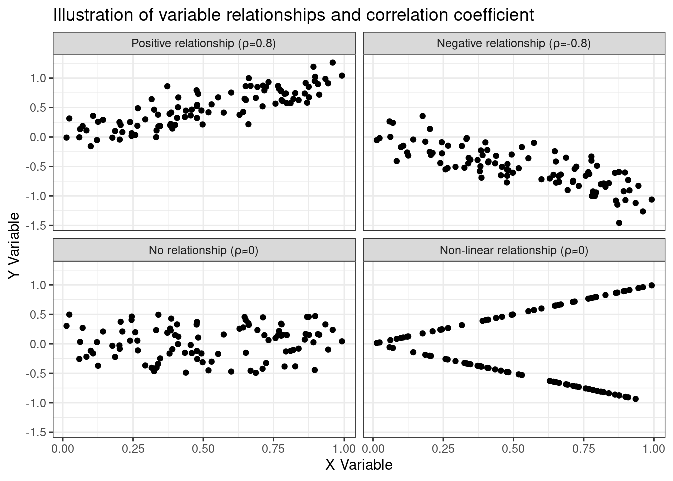
These examples were engineered to show various types of relationships and how they are reflected in the correlation coefficient. The two upper charts illustrate strong relationships: either positive (upper-left) or negative (upper-right).
The bottom-left chart shows no-relationships (these are just random numbers on the x and y-axis), and the bottom-right illustrates an interesting relationship: the two variables are not correlated (a correlation coefficient close to 0), but they are surely related to one another. The y-value can either be x or -x. A simple transformation of y (absolute value), would yield a correlation coefficient of 1 instead of 0. This last example also shows the limitation of using a correlation coefficient, having said that though, let’s use a correlogram to inspect the variables.
Correlograms to the rescue
A correlogram is a powerful tool that allows us to get a quick glimpse of the correlation coefficients of the data features visually. In our toy example, it looks like this:
corr_examples %>%
  set_names(c("Original variable", "Positive", "Negative", "No relationship", "Non-linear")) %>%
  cor() %>%
  ggcorrplot::ggcorrplot(ggtheme = theme_bw(),
                         title = 'Correlogram of the variables in our "toy example"',
                         colors = c("#FC8D59", "#FFFFFF", "#91CF60"))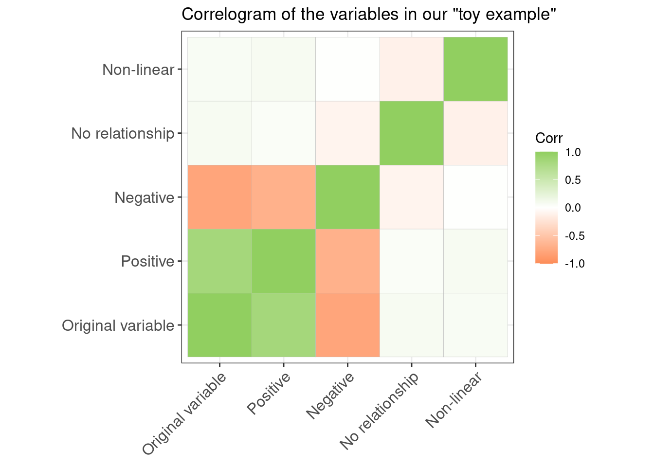
Using the correlogram, we can immediately see the relationships between our original variable, the positive and negative relationship variables. We can see that there are two variables with low correlation.
Now, let’s move to a more interesting and realistic example - illustrating movie-genera relationships.
Relationships of movie-genres
The IMDb has some interesting data for download (see this
link). Specifically, one of the files
they have made available is called title.basics.tsc.gz which contains
titles with information such as release dates, runtime (duration in
minutes), and associated genres. Since the original file is very large
in size, I have rearranged it to contain just the genres, with 0-1
coding (if a title is associated with a specific genre, the coding will
be 1, otherwise, it is 0).
library(tidyverse)

# Read the data
imdb_titles <- read_tsv('data.tsv')

# Have a look on what we have
glimpse(imdb_titles)

# Rework the data to extract the genres
imdb_genres  <- imdb_titles |>
   select(originalTitle, genres) |>
   separate(genres, into = c("genre1", "genre2", "genre3"), sep = ',')

# Make the data into a long format
imdb_genres_long <- imdb_genres |>
   pivot_longer(cols = -originalTitle, names_to = "gen_loc_rm", values_to = "genre") |>
   mutate(genre_assoc = 1) |>
   filter(!is.na(genre))

# Have a look on available genres in the data
imdb_genres_long  |>
   distinct(genre)

# Make it wide again - as preperation to the correlogram
imdb_genres_wide <- imdb_genres_long |>
   select(-gen_loc_rm) |>
   distinct(originalTitle, genre, .keep_all = TRUE) |>
   pivot_wider(id_cols = originalTitle,
               names_from = genre,
               values_from = genre_assoc,
               values_fill = 0) |>
   select(-`\\N`)

# Export the result to preserve for use
# This one exports the entire data with title names
# write_csv(imdb_genres_wide, "imdb_genre_association.csv")
# This one exports just the 0-1 encoding without title names (takes less space)
arrow::write_parquet(imdb_genres_wide |> select(-originalTitle),
   "imdb_genre_association_no_name.parquet")
imdb_genres_coding <- arrow::read_parquet("data/imdb_genre_association_no_name.parquet")
glimpse(imdb_genres_coding)## Rows: 4,701,772
## Columns: 28
## $ Documentary <dbl> 1, 0, 0, 0, 0, 0, 0, 1, 0, 1, 1, 1, 1, 0, 0, 1, 1, 0, 0, …
## $ Short <dbl> 1, 1, 0, 1, 1, 1, 1, 1, 0, 1, 1, 1, 1, 1, 1, 1, 1, 1, 1, …
## $ Animation <dbl> 1, 1, 1, 1, 0, 0, 0, 0, 1, 0, 0, 0, 0, 1, 1, 0, 0, 0, 0, …
## $ Comedy <dbl> 0, 0, 1, 0, 1, 0, 0, 0, 1, 0, 0, 0, 0, 1, 0, 0, 0, 0, 1, …
## $ Romance <dbl> 0, 0, 1, 0, 0, 0, 0, 0, 1, 0, 0, 0, 0, 0, 0, 0, 0, 0, 0, …
## $ Sport <dbl> 0, 0, 0, 0, 0, 0, 1, 0, 0, 0, 0, 0, 0, 0, 0, 0, 0, 0, 0, …
## $ News <dbl> 0, 0, 0, 0, 0, 0, 0, 0, 0, 0, 0, 0, 0, 0, 0, 0, 0, 0, 0, …
## $ Drama <dbl> 1, 0, 0, 0, 0, 0, 0, 0, 0, 0, 0, 0, 0, 1, 0, 0, 0, 0, 0, …
## $ Fantasy <dbl> 0, 0, 0, 0, 0, 0, 0, 0, 0, 0, 0, 0, 0, 0, 0, 0, 0, 0, 0, …
## $ Horror <dbl> 0, 0, 0, 0, 0, 0, 0, 0, 0, 0, 0, 0, 0, 0, 0, 0, 0, 0, 0, …
## $ Biography <dbl> 0, 0, 0, 0, 0, 0, 0, 0, 0, 0, 0, 0, 0, 0, 0, 0, 0, 0, 0, …
## $ Music <dbl> 0, 0, 0, 0, 0, 0, 0, 0, 0, 0, 0, 0, 0, 0, 0, 0, 0, 0, 0, …
## $ War <dbl> 0, 0, 0, 0, 0, 0, 0, 0, 0, 0, 0, 0, 0, 0, 0, 0, 0, 0, 0, …
## $ Crime <dbl> 0, 0, 0, 0, 0, 0, 0, 0, 0, 0, 0, 0, 0, 0, 0, 0, 0, 0, 0, …
## $ Western <dbl> 0, 0, 0, 0, 0, 0, 0, 0, 0, 0, 0, 0, 0, 0, 0, 0, 0, 0, 0, …
## $ Family <dbl> 0, 0, 0, 0, 0, 0, 0, 0, 1, 0, 0, 0, 0, 1, 0, 0, 0, 0, 0, …
## $ Adventure <dbl> 0, 0, 0, 0, 0, 0, 0, 0, 0, 0, 0, 0, 0, 0, 0, 0, 0, 0, 0, …
## $ Action <dbl> 1, 0, 0, 0, 0, 0, 0, 0, 0, 0, 0, 0, 0, 0, 0, 0, 0, 0, 0, …
## $ History <dbl> 0, 0, 0, 0, 0, 0, 0, 0, 0, 0, 0, 0, 0, 0, 0, 0, 0, 0, 0, …
## $ Mystery <dbl> 0, 0, 0, 0, 0, 0, 0, 0, 0, 0, 0, 0, 0, 0, 0, 0, 0, 0, 0, …
## $ `Sci-Fi` <dbl> 0, 0, 0, 0, 0, 0, 0, 0, 0, 0, 0, 0, 0, 0, 0, 0, 0, 0, 0, …
## $ Musical <dbl> 0, 0, 0, 0, 0, 0, 0, 0, 0, 0, 0, 0, 0, 0, 0, 0, 0, 0, 0, …
## $ Thriller <dbl> 0, 0, 0, 0, 0, 0, 0, 0, 0, 0, 0, 0, 0, 0, 0, 0, 0, 0, 0, …
## $ `Film-Noir` <dbl> 0, 0, 0, 0, 0, 0, 0, 0, 0, 0, 0, 0, 0, 0, 0, 0, 0, 0, 0, …
## $ `Talk-Show` <dbl> 0, 0, 0, 0, 0, 0, 0, 0, 0, 0, 0, 0, 0, 0, 0, 0, 0, 0, 0, …
## $ `Game-Show` <dbl> 0, 0, 0, 0, 0, 0, 0, 0, 0, 0, 0, 0, 0, 0, 0, 0, 0, 0, 0, …
## $ `Reality-TV` <dbl> 0, 0, 0, 0, 0, 0, 0, 0, 0, 0, 0, 0, 0, 0, 0, 0, 0, 0, 0, …
## $ Adult <dbl> 1, 0, 0, 0, 0, 0, 0, 0, 0, 0, 0, 0, 0, 0, 0, 0, 0, 0, 0, …The following correlogram shows the relationships between genres. It is also “clustered” in the sense that similar genres are re-arranged to appear as blocks.
imdb_cor <- cor(imdb_genres_coding)
ggcorrplot::ggcorrplot(imdb_cor,
                       title = "Correlogram of movie genres",
                       hc.order = TRUE,
                       ggtheme = theme_bw(),
                       colors = c("#D73027", "#FFFFFF", "#1A9850"),
                       tl.cex = 10,
                       tl.srt = 90) +
  theme(axis.text.x = element_text(vjust = 0.5))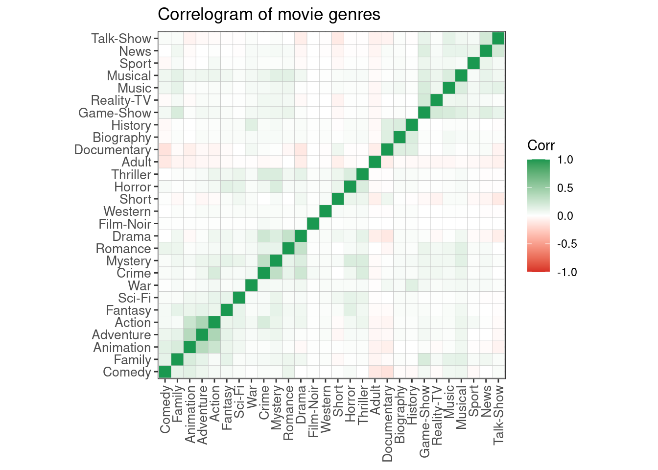
Although the correlations are not very strong between most genres (the highest are around 0.4 between action and adventure), the chart immediately highlights some positive relationships (partial list):
Action, Adventure, and Animation are related
History, Biography, and Documentary
Crime and Mystery
Romance and Drama
Talk-shows and News
Thriller and Horror (and also Crime and Mystery)
We can also see some negative (opposite) relationships such as:
Adult vs. Comedy
Documentary vs. Comedy
Drama vs. Documentary
Conclusions
In this post, I discussed correlations in general and illustrated how different relationships are expressed in positive, negative, or sometimes even low correlation (when the relationship is non-linear).
We’ve seen how correlogram charts can be a strong visual tool for quickly glancing at a large data set and highlighting some relationships.
Correlograms are usually only one of the initial steps - they give us some directions, but most of the time further research is required.