Settling class action lawsuits with conjoint analysis and R (+a conjoint shiny app)
A few days ago I presented at the 9th Israeli class action lawsuit conference. You’re probably asking yourself what would a data scientist do in a room full of lawyers?
Apparently, there is a lot to do… Here’s the story: being in market research, we get a lot of lawyers which are faced with class action lawsuits (either suing or being sued) - and they hire us to conduct research and estimate things like the size of the group for the class action, or the total damages applied on the group.
This time, we did something special. we conducted our own survey, with consumers in the general public in Israel. The goal was to rate various ways of getting compensation (after settling a class action lawsuit).
For that we used conjoint analysis. Conjoint is where you ask the survey participants a set of questions (five in our case). Each question has a number of alternatives (or packages) to choose from, and these are randomized per respondent. In our case we showed three packages, each package is defined by three parameters relating to how a consumer can get compensation in case of a class action being won:
- Push versus pull - do you have to ask for the compensation or would you get the notification/compensation without asking.
- The value of the compensation - tested at 4 levels (25, 50, 75, and 100 ILS)
- The method of delivery - as a complimentary product, a refund at next purchase, bank cheque, or credit card.
The thing about conjoint analysis is that when you diversify enough, you can then run various models to estimate the weight of each parameter, i.e., using logistic regression.
The data is available in the github repo, and the specific data is under the data folder.
#library(tidyverse)
class_action_conjoint <- read_csv("https://raw.githubusercontent.com/adisarid/class-action-IL-survey/master/data/20190130020529-SurveyExport-general_public-conjoint.csv",
                                  skip = 1,
                                  col_names =
                                    c("Response ID", "Set Number", "Card Number",
                                      "compensation_push_pull", "compensation_amount_ILS", "compensation_type",
                                      "score_selection"))
## Rows: 7020 Columns: 7── Column specification ────────────────────────────────────────────────────────
## Delimiter: ","
## chr (2): compensation_push_pull, compensation_type
## dbl (5): Response ID, Set Number, Card Number, compensation_amount_ILS, scor...
## ℹ Use `spec()` to retrieve the full column specification for this data.
## ℹ Specify the column types or set `show_col_types = FALSE` to quiet this message.glimpse(class_action_conjoint)## Rows: 7,020
## Columns: 7
## $ `Response ID` <dbl> 10, 10, 10, 10, 10, 10, 10, 10, 10, 10, 10, 10…
## $ `Set Number` <dbl> 1, 1, 1, 2, 2, 2, 3, 3, 3, 4, 4, 4, 5, 5, 5, 1…
## $ `Card Number` <dbl> 1, 2, 3, 1, 2, 3, 1, 2, 3, 1, 2, 3, 1, 2, 3, 1…
## $ compensation_push_pull <chr> "push", "push", "push", "push", "pull", "pull"…
## $ compensation_amount_ILS <dbl> 75, 50, 25, 100, 25, 100, 75, 100, 50, 25, 75,…
## $ compensation_type <chr> "another_product", "credit_cart", "bank_cheque…
## $ score_selection <dbl> 0, 0, 100, 0, 100, 0, 0, 0, 100, 0, 100, 0, 10…class_action_conjoint %>% count(compensation_push_pull)## # A tibble: 2 × 2
## compensation_push_pull n
## <chr> <int>
## 1 pull 3516
## 2 push 3504class_action_conjoint %>% count(compensation_amount_ILS)## # A tibble: 4 × 2
## compensation_amount_ILS n
## <dbl> <int>
## 1 25 1759
## 2 50 1761
## 3 75 1752
## 4 100 1748class_action_conjoint %>% count(compensation_type)## # A tibble: 5 × 2
## compensation_type n
## <chr> <int>
## 1 another_product 1391
## 2 bank_cheque 1410
## 3 coupon 1403
## 4 credit_cart 1415
## 5 refund_next_purchase 1401You can see that the different options are balanced (they should be - they were selected randomly) and that the number of observations is \(7,020\). This is because we had \(n=468\) respondents answering the conjoint question groups, each selecting best one out of three, with five such random sets (\(5*3*468=7020\)).
Logistic regression
The easiest (and most basic) way to start analyzing the conjoint data is with logistic regression. Note that I’m not endorsing this use of logistic regression in conjoint analysis, because nowadays it has become a standard to compensate for mixed effects (see package lme4). However, for the purposes of this post, I’m going to carry on with the simple glm which is sufficiently good for our illustration. In any case, my experience is that the models yield similar results in most cases.
glm_set <- class_action_conjoint %>%
  mutate(score_selection = score_selection/100) %>%
  mutate(compensation_push_pull = factor(compensation_push_pull,
                                         levels = c("pull", "push"),
                                         ordered = F),
         compensation_type = factor(compensation_type,
                                    levels =
                                      c("another_product",
                                        "refund_next_purchase",
                                        "coupon",
                                        "bank_cheque",
                                        "credit_cart"),
                                    ordered = F)) %>%
  select(-`Set Number`, -`Card Number`, -`Response ID`) %>%
  mutate(compensation_amount_ILS = factor(compensation_amount_ILS, levels = c(25, 50, 75, 100)))

conjoint_glm_model <- glm(data = glm_set %>%
      select(score_selection, compensation_push_pull, compensation_amount_ILS, compensation_type),
    formula = score_selection ~ .,
    family = binomial())
summary(conjoint_glm_model)
##
## Call:
## glm(formula = score_selection ~ ., family = binomial(), data = glm_set %>%
## select(score_selection, compensation_push_pull, compensation_amount_ILS,
## compensation_type))
##
## Deviance Residuals:
## Min 1Q Median 3Q Max
## -1.8635 -0.8111 -0.5139 0.8796 2.6557
##
## Coefficients:
## Estimate Std. Error z value Pr(>|z|)
## (Intercept) -3.49667 0.11341 -30.832 <2e-16 ***
## compensation_push_pullpush 0.74140 0.05807 12.767 <2e-16 ***
## compensation_amount_ILS50 1.01476 0.09385 10.813 <2e-16 ***
## compensation_amount_ILS75 1.73623 0.09224 18.823 <2e-16 ***
## compensation_amount_ILS100 2.40149 0.09281 25.876 <2e-16 ***
## compensation_typerefund_next_purchase 0.08431 0.10399 0.811 0.418
## compensation_typecoupon 1.10396 0.09588 11.514 <2e-16 ***
## compensation_typebank_cheque 1.53888 0.09473 16.245 <2e-16 ***
## compensation_typecredit_cart 1.89640 0.09586 19.782 <2e-16 ***
## ---
## Signif. codes: 0 '***' 0.001 '**' 0.01 '*' 0.05 '.' 0.1 ' ' 1
##
## (Dispersion parameter for binomial family taken to be 1)
##
## Null deviance: 8936.7 on 7019 degrees of freedom
## Residual deviance: 7295.6 on 7011 degrees of freedom
## AIC: 7313.6
##
## Number of Fisher Scoring iterations: 4Note how most variables (actually all but compensation_typerefund_next_purchase) are significant and with a positive estimate (i.e., odds ratio > 1). This means means that when a certain variable increases, the probability of choosing the package increases, i.e.:
- Passively getting the compensation (“Push”) is better than a required act to get the compensation (“pull”) .
- Any sum of money (50, 75, 100) is better than 25, in an increasing odds ratio.
- Most compensation types (credit card payback, bank cheque, coupon) are significantly better than a complimentary product.
Now comes the interesting part: for example, compare the following three packages. Try to guess which one is more attractive:
| Parameter | Package 1 | Package 2 | Package 3 |
|---|---|---|---|
| Push/Pull | Pull | Pull | Push |
| Return | Credit | Refund | Coupon |
| Price | 25 | 75 | 25 |
It is not that easy to determine between the three. In this situation there is no single strategy which is superior to the others, we can however plot these three packages with the logistic regression response and standard errors. First let’s put them all in a tibble (I also added the best and worst packages).
package_comparison <- tribble(
  ~package_name, ~compensation_push_pull, ~compensation_amount_ILS, ~compensation_type,
  "pkg1", "pull", 25, "credit_cart",
  "pkg2", "pull", 75, "refund_next_purchase",
  "pkg3", "push", 25, "coupon",
  "worst", "pull", 25, "another_product",
  "best", "push", 100, "credit_cart"
) %>%
  mutate(compensation_amount_ILS = factor(compensation_amount_ILS)) # need to convert to factor - which is how it is modeled in the glm.

predicted_responses <- predict(conjoint_glm_model, newdata = package_comparison, type = "response", se.fit = T)

# lets join these together

package_responses <- package_comparison %>%
  mutate(fit = predicted_responses$fit,
         se.fit = predicted_responses$se.fit)

package_responses
## # A tibble: 5 × 6
## package_name compensation_push_pull compensation_amou…¹ compe…² fit se.fit
## <chr> <chr> <fct> <chr> <dbl> <dbl>
## 1 pkg1 pull 25 credit… 0.168 0.0129
## 2 pkg2 pull 75 refund… 0.158 0.0122
## 3 pkg3 push 25 coupon 0.161 0.0129
## 4 worst pull 25 anothe… 0.0294 0.00324
## 5 best push 100 credit… 0.824 0.0123
## # … with abbreviated variable names ¹compensation_amount_ILS,
## # ²compensation_type# P.S. - excuse the "credit_cart" typo (I build the model that way, only then noticed...)
ggplot(package_responses %>% slice(1:3) , aes(x = package_name, y = fit)) +
geom_point() +
geom_errorbar(aes(ymin = fit - se.fit, ymax = fit + se.fit)) +
ggtitle("Package comparison (packages 1-3)", subtitle = "Error bars represent the SE") +
ylab("Predicted response (glm logit)") +
xlab("Package name") +
scale_y_continuous(labels = scales::percent_format(accuracy = 1))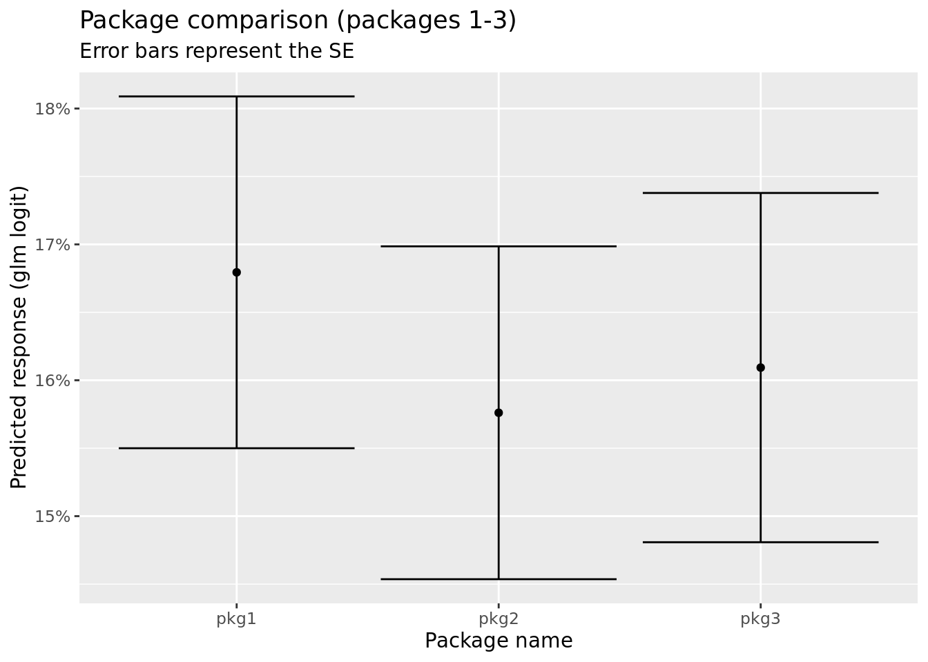
ggplot(package_responses, aes(x = package_name, y = fit)) +
  geom_point() +
  geom_errorbar(aes(ymin = fit - se.fit, ymax = fit + se.fit)) +
  ggtitle("Package comparison (including best and worst packages)", subtitle = "Error bars represent the SE") +
  ylab("Predicted response (glm logit)") +
  xlab("Package name") +
  scale_y_continuous(labels = scales::percent_format(accuracy = 1))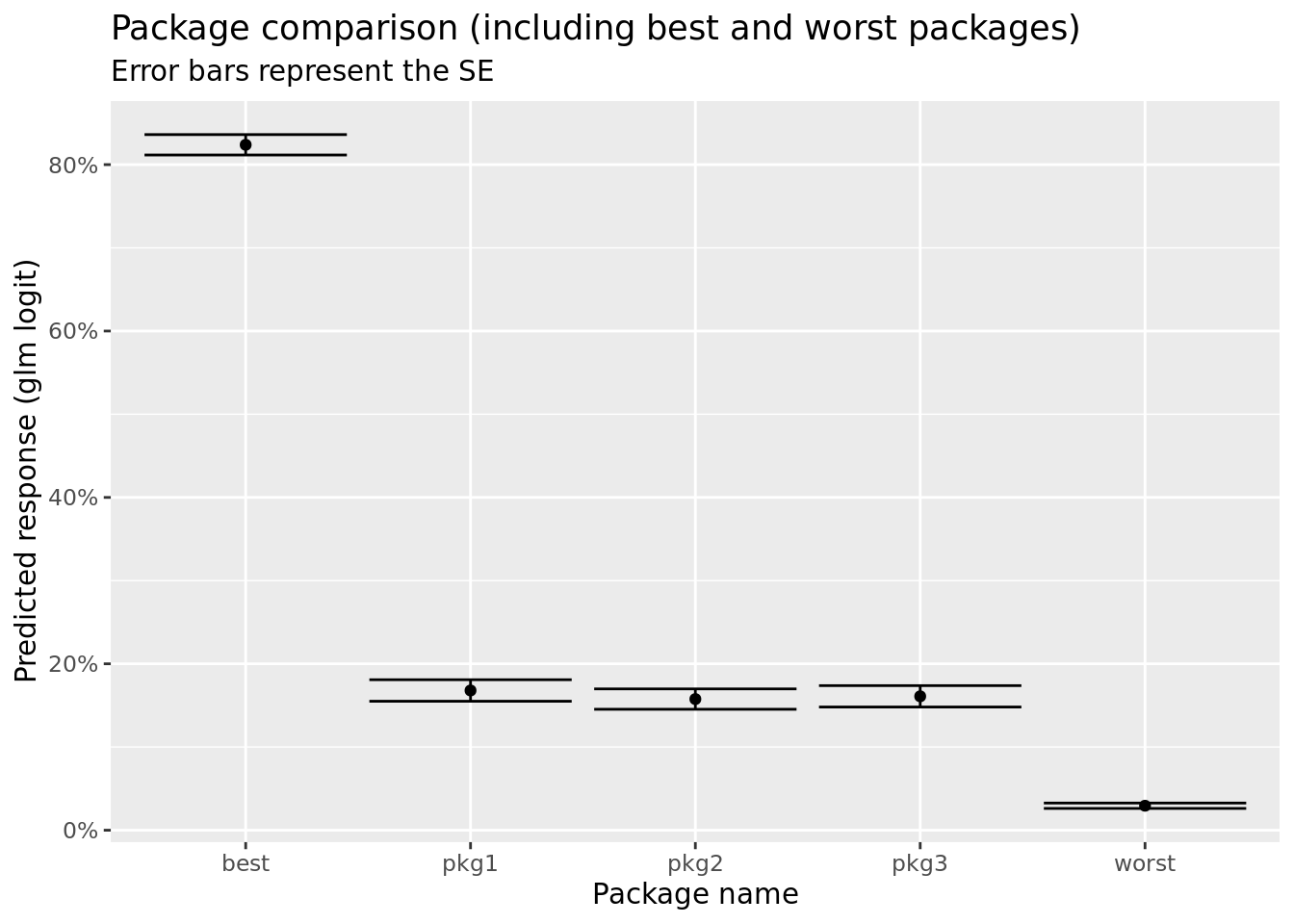
We see that the three packages (pkg1, pkg2, and pkg3) are relatively similar, within one standard error from one another. When compared to the worst package they are roughly \(\sim8\) times better (via odds ratio), but the best package is \(\sim5\) times better than packages 1-3.
One can use these concepts to illustrate the benefits of each parameter on the different packages, and let the user experience how different features make the packages more or less “attractive”.
As an experiment, I prepared a nice little shiny app which lets the user experiment with the different features: build two packages and then compare them. You can checkout the code at the github repo, or check out the live app here.
Conclusions
Surveys are a popular tool used in class actions (at least in Israel). They can be used to estimate the tradeoffs between various types of compensation or settlement, for example with the use of conjoint analysis.
With a glm model one can tell the differences of various packages, and the odds ratio is a way to illustrate to decision makers a comparison of various options (and how much “more attractive” is one package over another).
A shiny app can be a nice way to illustrate the results of a conjoint analysis, and to let the user experiment with how different features make a specific option better or worse than another option.